In this chapter, you will learn how to:
- Estimate a line of best fit and use it to make predictions.
- Interpret the slope and y-intercept in a statistical situation.
- Describe the form, direction, strength, and outliers of an association.
- Calculate residuals and create upper and lower bounds for predictions.
- Create residual plots and analyze them to determine whether a model is an appropriate fit to the data.
- Calculate the correlation coefficient and R2 and interpret them in context.
- Use mathematical terms to describe the form, direction, and strength of an association.
- Discover that association is not causation because there might be a lurking variable.
- Fit curved models to non-linear scatterplots.
|
Line of Best Fit: 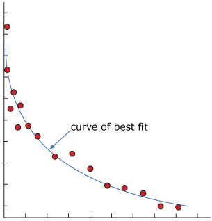
Residual Lines: We measure how far a prediction made by our model is from the actual observed value with a residual: residual = actual – predicted 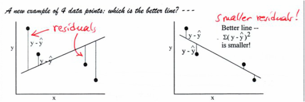
Upper and Lower Bounds: Green Lines = Upper and Lower Bounds
Black Line = LSRL 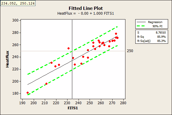
|
Least Squares Regression Line:
A unique best-fit line for data can be found by determining the line that makes the residuals, and hence the square of the residuals, as small as possible. We call this line the least squares regression line and abbreviate it LSRL. A calculator can find the LSRL quickly. Statisticians prefer the LSRL to some other best-fit lines because there is one unique LSRL for any set of data. 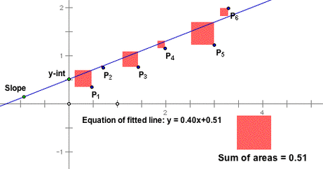
Interpreting Slope and y-Intercept:
The slope of a linear association plays the same role as the slope of a line in algebra. Slope is the amount of change we expect in the dependent variable (Δy) when we change the independent variable (Δx) by one unit. When describing the slope of a line of best fit, always acknowledge that you are making a prediction, as opposed to knowing the truth, by using words like “predict,” “expect,” or “estimate.” The y-intercept of an association is the same as in algebra. It is the predicted value of the dependent variable when the independent variable is zero. Be careful. In statistical scatterplots, the vertical axis is often not drawn at the origin, so the y-intercept can be someplace other than where the line of best fit crosses the vertical axis in a scatterplot. Also be careful about extrapolating the data too far—making predictions that are far to the right or left of the data. The models we create can be valid within the range of the data, but the farther you go outside this range, the less reliable the predictions become. When describing a linear association, you can use the slope, whether it is positive or negative, and its interpretation in context, to describe the direction of the association. |
Correlation Coefficient:
The correlation coefficient, r, is a measure of how much or how little data is scattered around the LSRL; it is a measure of the strength of a linear association. The correlation coefficient can take on values between −1 and 1. If r = 1 or r = −1 the association is perfectly linear. There is no scatter about the LSRL at all. A positive correlation coefficient means the trend is increasing (slope is positive), while a negative correlation means the opposite. A correlation coefficient of zero means the slope of the LSRL is horizontal and there is no linear association whatsoever between the variables.
